Estimating GC bias in short-read WGS data
A while ago at Edinburgh Genomics, we saw a phenomenon where some of the data we produced had significant inconsistency of coverage in genomic regions with high GC content. At the time, we only noticed it after we had finished generating the data, and it would have helped to have had an earlier warning of this so we could stop and resequence the sample. To this end, we implemented a GC bias estimate in our data processing.
GC bias
In most forms of whole genome sequencing we read the genome multiple times, giving us a coverage value for each base. If a sample has been sequenced to 30X coverage, each base has been read on average about 30 times. If you sequence a base at a given position 30 times and get an 'A' most times, then you can be pretty sure it's an 'A'. Ideally, we would sequence the whole genome to the same coverage all the way across, but due to the stochastic nature of the sequencing process, coverage is rarely completely even across the genome. On top of this natural randomness, coverage can in some cases be diminished in certain genomic regions such as those with extremes of GC content, which can affect analysis of quantitative features like copy number variation, but also basic variant detection.
A major source of GC bias in WGS library preparation is PCR amplification, which is a very useful technique for obtaining sequenceable DNA from small samples, but is also infamous among students, postdocs and professors alike for going wrong in a variety of ways, including inferior amplification of DNA fragments with particularly high or low GC content. If the sequence or GC content of the DNA fragments are known, it is possible to use additives and/or tune the PCR thermal cycling accordingly, but this is not possible in short-read sequencing where these are not known. As a result, the performance of the amplification is skewed by the different annealing temperatures of AT- and GC-rich DNA, and the tendency of GC-rich DNA to form stem loops. PCR-free library preparation has been seen to improve downstream processing of samples with high GC content.
In reality there is always some GC bias even in good short-read data, but here we were observing drops in coverage even in areas of moderately high GC for some library preps. For an example, see the plots below, generated from picardtools:
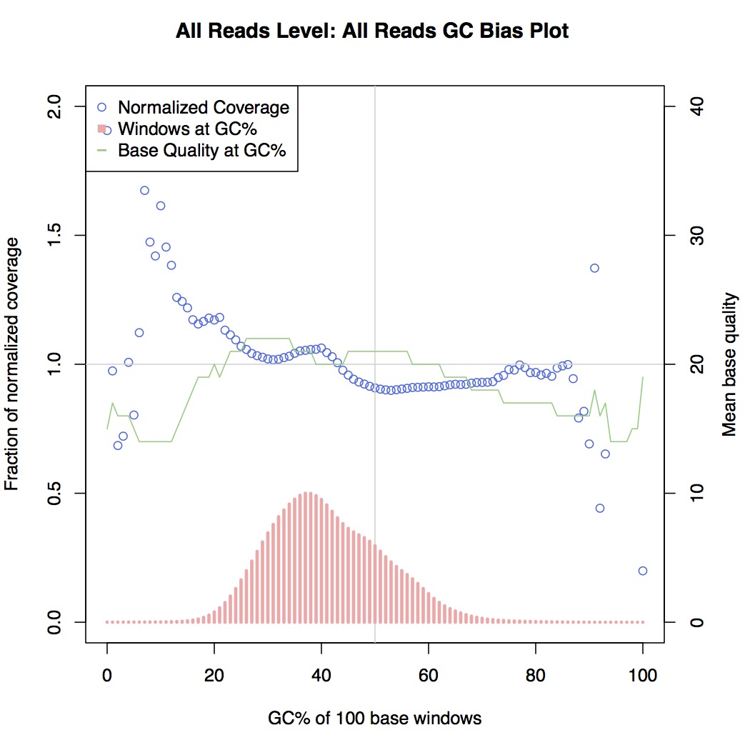
Non GC-biased
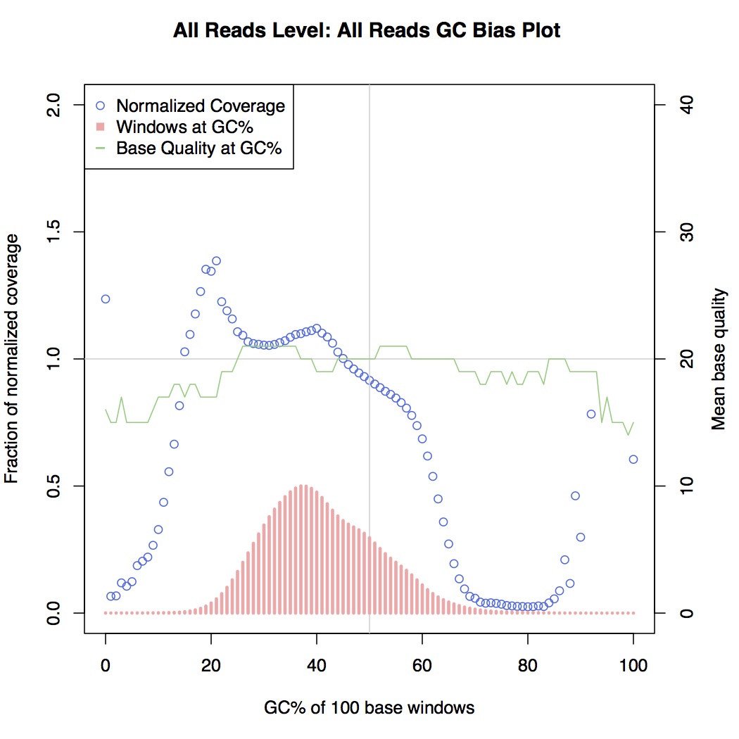
GC-biased
Here, coverage metrics are collected for areas along the sequenced genome and grouped by GC content bins, i.e. areas that are 0% GC, 1% GC, 2% GC, etc. all the way up to 100%. What distinguishes the GC-biased sample here is the drop-off in normalised coverage (the blue series) between 20% and 80% GC, which is otherwise relatively level in non-biased samples.
So to check for GC bias, we could generate one of these plots for each sample we sequence and look at it. However, this would not be an appropriate solution for us due to the large numbers of samples we process, so a better solution would be to extract a simple metric from the graph, apply a threshold to it and programatically flag up any samples that exceed it.
Theil-Sen estimation
The first metric we calculated was the mathematical equivalent of what we had been doing before, i.e. looking at the graph and checking whether coverage drops off at higher GC content. This would involve drawing a line of best through the data points and measuring its gradient. To do this, we used Theil-Sen estimation, which is implemented in SciPy. This algorithm essentially draws a line of best fit (shown below in red) through the input data points and returns a slope/gradient value:
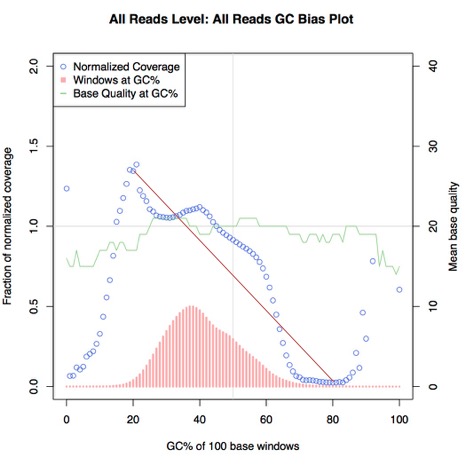
Theil-Sen estimation
If this value is sufficiently low or high (i.e. the line is steep enough), then we can interpret this as significant GC bias. We filtered the data points used in this estimation to only those between 20% and 80% GC, both because of the large amount of noise in the data outside this region skewing the metric, and because there is a precedence for this practice in the form of deeptools computeGCBias.
Deviation from normal
This is not a commonly-used statistical test as far as I am aware, but we decided to try it alongside Theil-Sen estimation to see if it was also an effective measurement. For each data point, we subtracted the normal from the absolute of the coverage value, which is effectively the equivalent of taking a ruler and measuring the distance on the graph between the data point and the normal - again shown below in red:
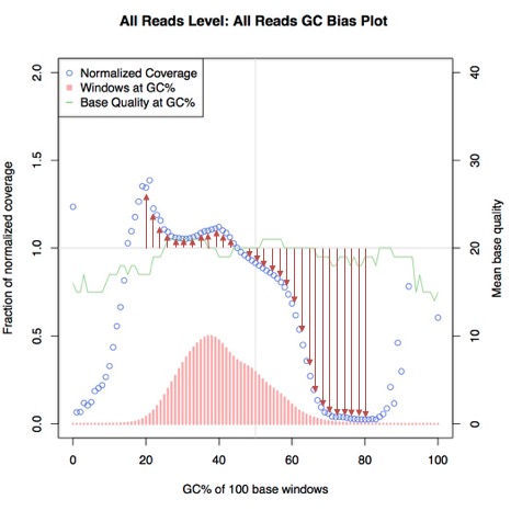
Normal deviation
This gives us a set of deviation values, which we can then take an average of. We did however use a different way
of filtering which data points to use. In Theil-Sen, we simply took all data points between 20% GC and 80% GC
whereas here, we used the 'windows' value for each data point, visible on the graphs above as the red series - if
the number of windows for a data point accounted for more than a certain fraction 1/n of the total windows in the
dataset, then it was included. The number n was calibrated to filter to a similar number of data points as when
performing simple filtering between 20% GC and 80% GC, and we arrived at a number of 2500.
Test data
We had a test set of 40 samples, 10 of which we knew from downstream analysis to be GC-biased. We were able to implement the core logic of our GC bias checks as below:
from scipy.stats.mstats import theilslopes

def theil_sen_estimate(lines):
    data_points = []
    for l in lines:
        if 20 <= int(l['GC']) <= 80:
            data_points.append(float(l['NORMALIZED_COVERAGE']))

    return theilslopes(data_points)

def deviation_from_normal(lines):
    total_diff = 0
    total_windows = sum([int(l['WINDOWS']) for l in lines])
    threshold = total_windows * 0.0004  # one 2500th of total_windows
    data_points = 0

    for l in lines:
        if int(l['WINDOWS']) > threshold:
            data_points += 1
            diff = abs(1 - float(l['NORMALIZED_COVERAGE']))
            total_diff += diff

    return total_diff / data_points
Results
Running the above algorithms on our 40 samples gave the following violin plots:
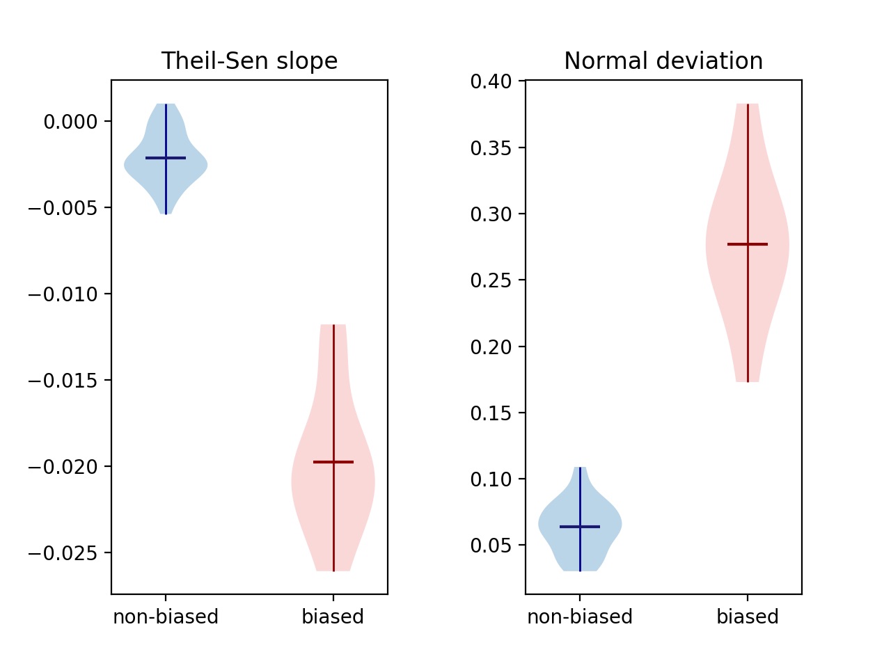
Violin plots of both metrics discussed above, for known biased/unbiased samples
For both metrics, biased samples are clearly separated from non-biased, differing by an order of magnitude. This shows that 1) it is possible to distinguish GC-biased from non GC-biased samples with a single metric, and 2) the deviation from normal is equally as effective a metric as Theil-Sen estimation.
The two metrics use different ways of filtering which data points to use. Filtering on GC content between 20% and 80% is consistent with the way other tools like deeptools computeGCBias filter data, whereas filtering on number of windows filters out noise in a way that's more agnostic of what the extremes are.
In reality, we use both of these metrics and rather than being a definite indicator of GC bias in a single sample, we intend to use them to identify trends in batches of samples processed together. For example, if many samples are prepared for sequencing together and all show different slopes or normal deviations, it is possible that there was a problem with the library preparation.
Having found a way of reporting on GC bias in samples, the next step is to find a way of comparing all samples in a library preparation plate, which our system is not currently optimised for. Once we have made this possible though, we will be able to detect biased library preparation in a sequencing batch, allowing us to repeat the preparation and sequencing in order to produce better data.
External links
-
Oyola et al, BMC Genomics 2012 (13:1): https://bmcgenomics.biomedcentral.com/articles/10.1186/1471-2164-13-1
Paper describing general PCR bias against both GC-rich and AT-rich DNA, and the solutions for them
-
Varadaraj & Skinner, Gene 1994 (140:1, 1-5): https://www.ncbi.nlm.nih.gov/pubmed/8125324?dopt=Abstract&holding=npg
Improving performance of GC-rich PCR by using reagents to prevent formation of secondary structures
-
McDowell et al, Nucleic Acids Research 1998 (26:14, 3340-7): https://www.ncbi.nlm.nih.gov/pubmed/9649616?dopt=Abstract&holding=npg
Effect of high melting points on PCR performance
-
Mamedov et al, Computational Biology and Chemistry 2008 (32:6): https://www.sciencedirect.com/science/article/pii/S1476927108000881
Tuning of PCR thermal cycling for GC-rich DNA
-
Kozarewa et al, Nature Methods 2009 (6:4, 291-295): https://www.ncbi.nlm.nih.gov/pubmed/19287394
PCR-free Illumina library preparation
-
Dohm et al, Nucleic Acids Research 2008 (36:16, e105): https://www.ncbi.nlm.nih.gov/pmc/articles/PMC2532726
Miscalls in sequencing of high-GC DNA
-
Nakamura et al, Nucleic Acids Research 2011 (39:13, e90): https://www.ncbi.nlm.nih.gov/pmc/articles/PMC3141275
Another paper discussing sequencing miscalls in GC-rich DNA